1. Biological Fundamentals

1.1. Neuron Definition

Neurons are the fundamental unit of the nervous system specialized to transmit information to different parts of the body.

1.2. What is a Nueron?

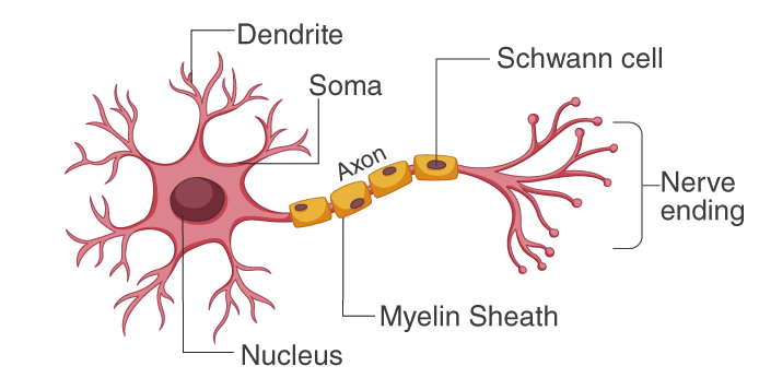
Neurons are the fundamental units of the nervous system. They receive signals and send them to different parts of the body. This process involves both physical and electrical pathways. Various neuron types assist in transmitting information, including sensory neurons, motor neurons, and interneurons.

structure-of-neuron

The sensory neurons carry information from the sensory receptor cells throughout the body to the brain. Meanwhile, motor neurons transmit information from the brain to the muscles. The interneurons transmit information between different neurons in the body.

The most important concepts that we need to relate to the Perceptron are:

Dendrites: These are the branches of the neuron that receive signals from other neurons. They are the input part of the neuron.
Axon: This is the long, thin part of the neuron that carries signals to other neurons. It is the output part of the neuron.
Nucleus: This is the part of the neuron that contains the genetic material. It is the control center of the neuron.

2. What is the Perceptron?

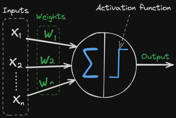
The Perceptron is a simple algorithm that can be used to classify data into two categories. It is a type of artificial neural network that is used in supervised learning. The Perceptron is a linear classifier, which means that it can only be used to classify data that is linearly separable. This means that the data can be separated into two categories by a straight line.

perceptron

The Perceptron works by taking a set of input values:

x_{1}, x_{2}, ..., x_{n}

and multiplying them by a set of weights:

x_{1} * w_{1} + x_{1} * w_{2} + ... + x_{1} * w_{n}

writing the sum compactly with summation notation as:

\sum_{i = 1}^{i = n} x_{i} * w_{i}

It then adds these values together and passes the result through an activation function. The activation function is used to determine the output of the Perceptron. If the output is greater than a certain threshold, the Perceptron will output a 1, otherwise it will output a 0. The diagram has as example Binary Step Function as the activation function.

f(x) = \left\{\begin{matrix} 0 for x < 0\\ 1 for x\geqslant 1 \end{matrix}\right.

The Perceptron is trained by adjusting the weights until it correctly classifies the input data. This is done by comparing the output of the Perceptron to the expected output and adjusting the weights accordingly.

3. Working with credit score

3.1. What is a Credit Score?

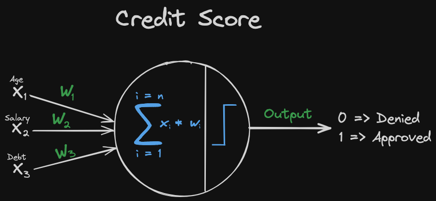
A credit score is a numerical representation of a person’s creditworthiness. It is used by lenders to determine whether or not to extend credit to a person. In this case, we are going to use age, salary and debt as input values to the Perceptron.

perceptron-credit-score

3.2. Writing the Perceptron Algorithm

The Perceptron algorithm can be written in Python as follows:

3.2.1. Importing Libraries and create a dataset

We are going to create a dataset of ten people with their age, salary, and debt. We are also going to create an expected output for each person. The expected output is 0 if the person has a good credit score and 1 if the person has a bad credit score.

import numpy as np
import matplotlib.pyplot as plt

# Dataset of ten people -> [age, salary]
dataset = np.array([
    [22, 60000],
    [25, 58801],
    [30, 70000],
    [35, 93500],
    [40, 120000],
    [45, 95000],
    [50, 110000],
    [55, 120000],
    [58, 29491],
    [62, 73679]
])

# Normalize the dataset. -1 to 1
scaler = StandardScaler()
dataset = scaler.fit_transform(dataset)

# Expected output
expected_output = np.array([0, 0, 0, 1, 1, 1, 1, 1, 0, 1])

Normalized dataset:

array([[-1.51252526, -0.81714392],
       [-1.2878928 , -0.85965493],
       [-0.91350536, -0.46259002],
       [-0.53911792,  0.37061165],
       [-0.16473047,  1.31017949],
       [ 0.20965697,  0.42379473],
       [ 0.58404441,  0.95562558],
       [ 0.95843185,  1.31017949],
       [ 1.18306432, -1.89885242],
       [ 1.48257427, -0.33214964]])

3.2.2. Scatter plot of the dataset

We are going to create a scatter plot of the dataset to see how the data is distributed.

# Scatter plot of the dataset
plt.scatter(dataset[:5, 0], dataset[:5, 1], color='b', label='Good Credit Score')
plt.scatter(dataset[5:, 0], dataset[5:, 1], color='r', label='Bad Credit Score')
plt.xlabel('Age')
plt.ylabel('Salary')
plt.legend()
plt.show()

3.2.3. Activation function and Perceptron algorithm

For this example, we are going to use the tanh activation function. The tanh function is a hyperbolic tangent function that maps the input to the range (-1, 1). The Perceptron algorithm is going to use the tanh function to classify the data.

# Activation function
def activation_function(x):
    return np.tanh(x)

3.2.4. Perceptron algorithm

The Perceptron algorithm is used to train the Perceptron by adjusting the weights until it correctly classifies the input data. This is done by comparing the output of the Perceptron to the expected output and adjusting the weights accordingly. The parameters of the algorithm are the dataset, the expected output, the learning rate, and the number of epochs.

Dataset: The dataset of input values.
Expected output: The expected output for each input value.
Learning rate: The learning rate is used to control how much the weights are adjusted during training.
Epochs: The number of epochs is the number of times the Perceptron is trained on the dataset.

# Perceptron algorithm
def perceptron_algorithm(dataset, expected_output, learning_rate, epochs):
    # Random weights with 3 elements (2 for the dataset and 1 for the bias)
    weights = np.random.rand(3)
    # List to store the errors
    errors = []

    # Epochs define how many times the algorithm will run
    for epoch in range(epochs):
        total_error = 0
        # Iterate over the dataset
        for i in range(len(dataset)):
            # Insert the bias into the dataset
            x = np.insert(dataset[i], 0, 1)
            # Calculate the output using the activation function
            y = activation_function(np.dot(x, weights))
            # Calculate the error using the expected output
            error = expected_output[i] - y
            # Update the weights
            weights += learning_rate * error * x
            # Sum the error to the total error
            total_error += error
        # Print the epoch, input, weights, output and error
        print(f"Epoch {epoch + 1}/{epochs}, x: {x}, weights: {weights}, y: {y}, error: {error}")
        # Append the total error to the errors list
        errors.append(total_error)
    return weights, errors

3.2.5. Training the Perceptron

We are going to train the Perceptron using the dataset and the expected output. We are going to use a learning rate of 0.1 and 100 epochs.

# Training the Perceptron
learning_rate = 0.1
epochs = 100
weights, errors = perceptron_algorithm(dataset, expected_output, learning_rate, epochs)

3.2.6. Plotting the errors

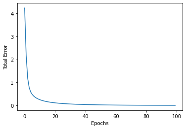
We are going to plot the errors to see how the Perceptron is trained.

# Plotting the errors
plt.plot(errors)
plt.xlabel('Epochs')
plt.ylabel('Total Error')
plt.show()

perceptron-credit-score-errors

By analyzing the errors plot, we can observe that the errors were significantly reduced up to 40 epochs. However, after that point, there is a possibility of overfitting occurring. We can adjust the learning rate and the number of epochs to improve the performance of the Perceptron.

3.2.7. Testing the Perceptron

We are going to test the Perceptron using the same dataset. We are going to compare the output of the Perceptron to the expected output to see how well the Perceptron has been trained.

In this code snippet, we start by creating an array named new_person that contains the data for a new individual. The data in this case represents the age (33) and the salary (80000) of the individual.

Following this, we normalize the data using the same scaler object that was used for normalizing the training data. It’s crucial to use the same scaler object to ensure consistency in the way the data is transformed.

Once the data is normalized, we insert a 1 at the start of the normalized array. This 1 represents the bias in the perceptron model, which provides the model with the flexibility to shift the activation function either to the left or right.

Next, we calculate the dot product of this array and the weights of the model, and pass the result to the activation function. The output of this function, y, is the predicted classification for the new individual.

Finally, we print the array x and the output y. We also print whether the person is “Accepted” or “Not accepted” based on the value of y.

# Testing the Perceptron
new_person = np.array([33, 80000])
new_person = scaler.transform([new_person])
x = np.insert(new_person[0], 0, 1)
y = activation_function(np.dot(x, weights))
print(f"Test, x: {x}, y: {y}")
# Print if the person is accepted or not
print("Accepted" if y > 0 else "Not accepted")

The output of the code snippet is as follows:

Test, x: [ 1.         -0.68887289 -0.10803612], y: 0.7551224205565439
Accepted

The output of the Perceptron is 0.755, which is greater than 0. This means that the Perceptron has classified the new individual as having a bad credit score.

4. Conclusion

To get code snippets and more details about the Perceptron, you can check the Notebook Github.

The Perceptron - An Artificial Neural Network to Classify Data